
Battery Life Calculation for Pulse-Driven Embedded Systems
Battery life math has a reputation for being simple. Capacity divided by current. Done. Ship it.
That works right up until it doesn’t.
The reason detailed power characterization matters is that small misunderstandings in current assumptions and battery capacity can turn into multi-year errors in lifetime projections. To avoid that, we have to start with the battery itself.
Battery characteristics and behaviors vary widely by chemistry, environmental conditions, and load behavior. One important factor that almost all batteries have in common is internal resistance. When a load is applied to a cell, the terminal voltage sags. This voltage sag can be modeled as a resistance in series with the voltage source.
As the battery becomes depleted, this effective internal resistance increases. The result is greater voltage sag for the same applied load. Embedded systems typically contain electronics with a strict minimum operating voltage, often called the brownout voltage. Once the battery reaches a point where the next load pulse causes the terminal voltage to dip below this threshold, the battery is effectively dead for that application—even if charge remains.
In pulse-driven systems, especially radio transmitters, this condition can occur well before the nameplate capacity has been exhausted.
Usable Battery Capacity
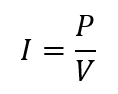
In some applications, the load behaves closer to a constant-power sink than a constant-current sink. In this case, as the terminal voltage drops, current increases to maintain power:
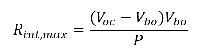
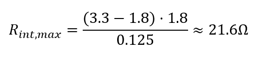
 If we model the battery as a Thevenin source with open-circuit voltage V_ocin series with internal resistance R_int, then at the brownout threshold V_bo, the maximum allowable internal resistance is determined by the condition that the terminal voltage under load equals the brownout voltage.
At brownout:
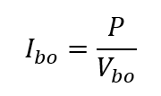 Substituting:
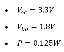
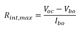 For a radio transmitting at 38mA from a 3.3V rail, the instantaneous pulse power is approximately:
 With:
With:
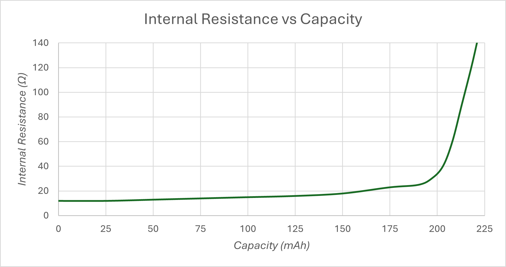
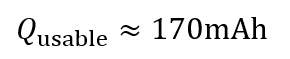
 Some battery manufacturers are kind enough to include a plot of internal resistance by SOC. Reviewing the internal resistance curve in Figure 1, we see that the CR2032 reaches approximately 22Ω at around 170mAh of discharged capacity. This establishes the usable capacity from a pulse-sag perspective.
Figure 1
 In other words, this system is pulse-limited, not capacity-limited.
Integrating the Real Load
The next step is determining how quickly that usable charge is consumed. This is where an accurate measurement and characterization of actual discharge events becomes critical. See the discharge waveform in Figure 2 with the device operating at 3.3V.
Figure 2
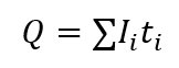
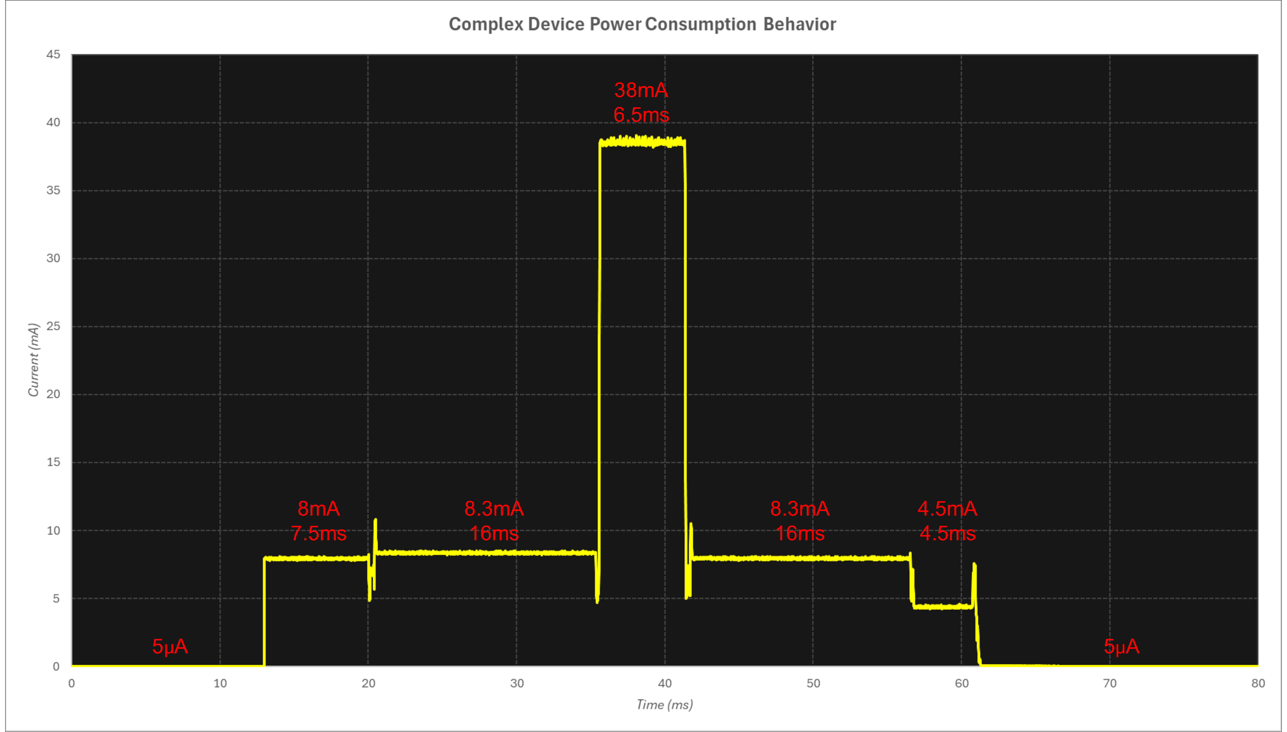 The measured waveform decomposes the device behavior into discrete states: wake, processing, transmit, receive, cleanup, and long-duration sleep. Each segment has a known current and duration. The table converts those into charge per occurrence and then scales by event frequency to obtain charge per hour. Rather than guessing at an “average current,” we integrate the actual behavior:
 scaled by how often the event repeats. With that number in hand, battery life becomes:
 Knowing that this waveform repeats once every ten minutes, we can ingest each of the components of this event into the equation and compute an estimated battery life of 3.24 years as shown in Figure 3.
Figure 3
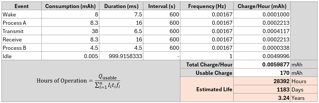 Note the Idle event. This is the current consumption of the device in sleep mode, when no other events are taking place. As such, the duration of this event is the inverse of the sum of the duration of all other events in the table.
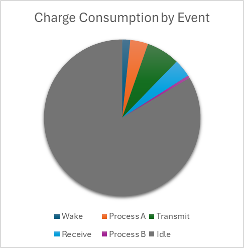
 In this particular case, although transmit pulses define usable capacity, the 5µA idle current dominates charge consumption rate, as shown in Figure 4.
Figure 4
Other Considerations
Internal resistance depends on pulse width, temperature, and state of charge. The IR curve in Figure 1 corresponds to specific test conditions; different pulse widths will shift the effective impedance.
Cold temperatures significantly increase impedance and reduce usable capacity. A design that works at 22°C may brown out at −10°C.
Retry behavior increases pulse frequency. Since high-current events scale directly with retry count, poor link conditions shorten battery life.
If a buck or boost converter is added later, battery current will differ from load current. Efficiency varies with input voltage and load, introducing drift over battery life.
Manufacturing variation matters. A sleep current shift from 5 µA to 7 µA reduces multi-year lifetime in measurable ways.
Primary lithium self-discharge is typically 1–2% per year at room temperature. In systems drawing microamps continuously, this is usually a second-order effect, but it becomes relevant in ultra-low-duty-cycle designs approaching shelf-life limits.
Conclusion
The process is simple but not simplistic.
- Measure the waveform
- Break it into segments
- Integrate current over time
- Scale by event frequency
- Apply margin for temperature, voltage sag, and real-world variability
Battery life is not a guess. It is an integral. The math itself is straightforward. The nuance is in measuring the right things – and accepting that the battery does not care about the number printed on its label.
Once you start treating it that way, your products start behaving the way you promised they would.